ffsimulator runs simulations on a given fantasy league based that league’s rosters, scoring settings, and current redraft rankings, connecting this data to historical weekly performances for each (preseason) positional ranking.
This vignette will introduce the basic usage of ffsimulator - you may also be interested in the motivations and custom simulations vignettes!
Usage - Simulating Seasons
ffsimulator connects directly to your league (via the ffscrapr package) and can be used at a high level with just a few lines of code:
foureight_conn <- mfl_connect(2021, 22627)

foureight_sim <- ff_simulate(conn = foureight_conn, n_seasons = 10, n_weeks = 14)
foureight_sim
#> <ff_simulation: 10 simulated seasons of Four-Eight Dynasty League>
#> List of 7
#> $ summary_simulation: tibble [12 × 11] (S3: tbl_df/tbl/data.frame)
#> $ summary_season : tibble [120 × 12] (S3: tbl_df/tbl/data.frame)
#> $ summary_week : tibble [1,680 × 16] (S3: tbl_df/tbl/data.frame)
#> $ roster_scores :Classes 'data.table' and 'data.frame': 51450 obs. of 23 variables:
#> $ projected_scores :Classes 'data.table' and 'data.frame': 51450 obs. of 14 variables:
#> $ league_info : tibble [1 × 17] (S3: tbl_df/tbl/data.frame)
#> $ simulation_params : tibble [1 × 9] (S3: tbl_df/tbl/data.frame)ffsimulator includes a few automatic plots that can be run on this ff_simulation object to get a quick sense of the simulation output:
plot(foureight_sim) # defaults to type = "wins"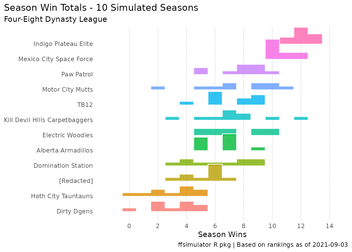
plot(foureight_sim, type = "rank")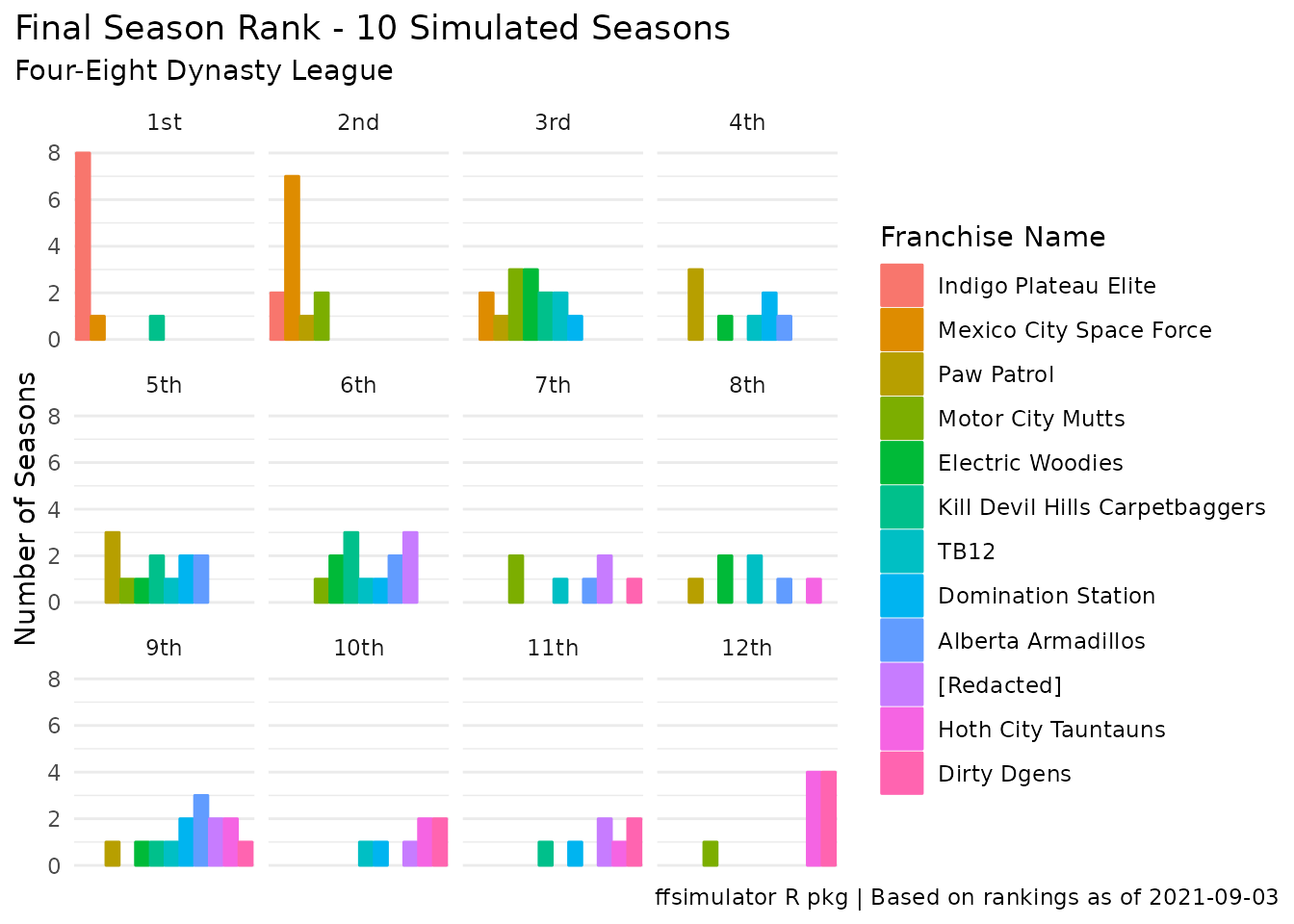
plot(foureight_sim, type = "points")
#> Picking joint bandwidth of 7.68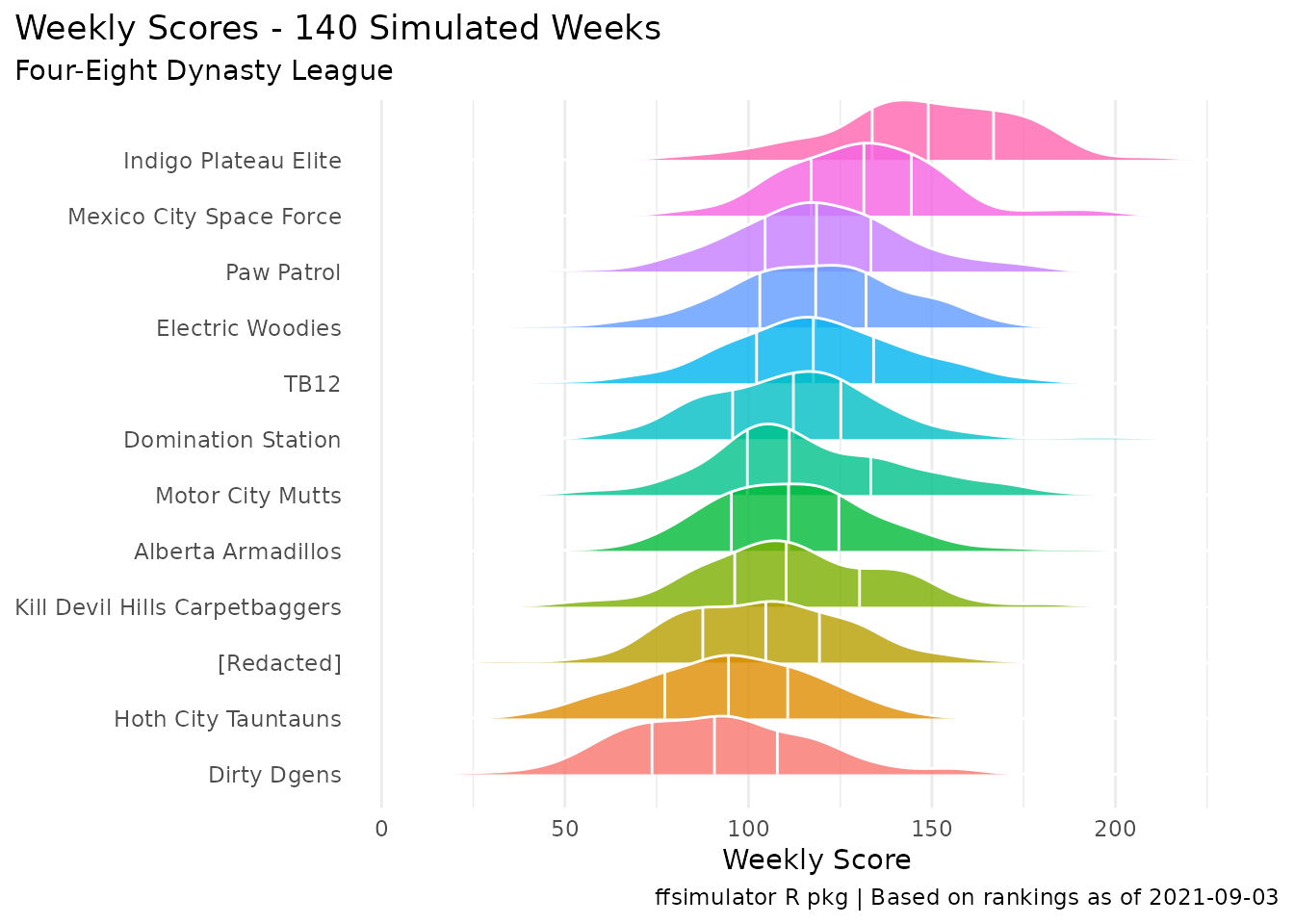
You can also access the various component dataframes by name, for further analysis.
The summary_simulation table is a team-level summary across all of the simulated seasons.
foureight_sim$summary_simulation
#> # A tibble: 12 × 11
#> league_id franchise…¹ franc…² seasons h2h_w…³ h2h_w…⁴ allpl…⁵ allpl…⁶ point…⁷
#> <chr> <chr> <chr> <int> <dbl> <dbl> <dbl> <dbl> <dbl>
#> 1 22627 0012 Indigo… 10 12.1 0.864 134. 0.867 2074.
#> 2 22627 0001 Mexico… 10 10.6 0.757 110 0.714 1842.
#> 3 22627 0007 Paw Pa… 10 7.8 0.557 84.9 0.551 1671.
#> 4 22627 0004 Electr… 10 7.4 0.529 84.2 0.547 1649.
#> 5 22627 0011 TB12 10 7.1 0.507 83.5 0.542 1659.
#> 6 22627 0005 Motor … 10 7.6 0.543 79.2 0.514 1626.
#> 7 22627 0009 Kill D… 10 7.3 0.521 74.8 0.486 1570.
#> 8 22627 0008 Domina… 10 6.3 0.45 73.6 0.478 1571.
#> 9 22627 0003 Albert… 10 6.4 0.457 71.4 0.464 1568.
#> 10 22627 0010 [Redac… 10 5.3 0.379 54.9 0.357 1458.
#> 11 22627 0006 Hoth C… 10 3 0.214 38.3 0.249 1318.
#> 12 22627 0002 Dirty … 10 3.1 0.221 35.7 0.232 1277.
#> # … with 2 more variables: points_against <dbl>, potential_points <dbl>, and
#> # abbreviated variable names ¹franchise_id, ²franchise_name, ³h2h_wins,
#> # ⁴h2h_winpct, ⁵allplay_wins, ⁶allplay_winpct, ⁷points_for
#> # ℹ Use `colnames()` to see all variable namesThe summary_season table is a season-level summary of all weeks within those seasons - any one of these seasons “could” theoretically be the outcome of the upcoming season!
foureight_sim$summary_season
#>      season league_id franchise_id                 franchise_name h2h_wins
#>   1:      1     22627         0001        Mexico City Space Force       12
#>   2:      1     22627         0002                    Dirty Dgens        0
#>   3:      1     22627         0003             Alberta Armadillos        5
#>   4:      1     22627         0004               Electric Woodies        7
#>   5:      1     22627         0005               Motor City Mutts       10
#>  ---
#> 116:     10     22627         0008             Domination Station        5
#> 117:     10     22627         0009 Kill Devil Hills Carpetbaggers       12
#> 118:     10     22627         0010                     [Redacted]        7
#> 119:     10     22627         0011                           TB12        8
#> 120:     10     22627         0012           Indigo Plateau Elite       11
#>      h2h_winpct allplay_wins allplay_games allplay_winpct points_for
#>   1:      0.857          125           154          0.812   2034.086
#>   2:      0.000           27           154          0.175   1187.849
#>   3:      0.357           63           154          0.409   1524.148
#>   4:      0.500           71           154          0.461   1579.101
#>   5:      0.714           80           154          0.519   1635.749
#>  ---
#> 116:      0.357           64           154          0.416   1460.263
#> 117:      0.857           88           154          0.571   1629.849
#> 118:      0.500           65           154          0.422   1490.238
#> 119:      0.571          100           154          0.649   1727.765
#> 120:      0.786          133           154          0.864   2066.457
#>      points_against potential_points
#>   1:       1622.343          2631.29
#>   2:       1798.732          1502.92
#>   3:       1543.897          1947.87
#>   4:       1694.826          2064.90
#>   5:       1519.509          2138.25
#>  ---
#> 116:       1555.725          1901.09
#> 117:       1403.566          2075.04
#> 118:       1469.356          1896.33
#> 119:       1601.649          2215.87
#> 120:       1485.318          2732.65
The summary_week table is a week-level summary of each team’s performance, including the optimal lineup that could have been played by the team and the randomly-generated lineup efficiency factor:
foureight_sim$summary_week
#>       season season_week                 franchise_name optimal_score
#>    1:      1           1        Mexico City Space Force        166.65
#>    2:      1           1                    Dirty Dgens        145.65
#>    3:      1           1             Alberta Armadillos        108.13
#>    4:      1           1               Electric Woodies        166.51
#>    5:      1           1               Motor City Mutts        148.63
#>   ---
#> 1676:     10          14             Domination Station        182.70
#> 1677:     10          14 Kill Devil Hills Carpetbaggers        175.64
#> 1678:     10          14                     [Redacted]        134.50
#> 1679:     10          14                           TB12         64.17
#> 1680:     10          14           Indigo Plateau Elite        205.99
#>       lineup_efficiency team_score opponent_score result
#>    1:             0.691    115.169         76.084      W
#>    2:             0.737    107.286        132.011      L
#>    3:             0.776     83.912        179.982      L
#>    4:             0.793    132.011        107.286      W
#>    5:             0.682    101.357        143.900      L
#>   ---
#> 1676:             0.740    135.286        113.904      W
#> 1677:             0.795    139.638        100.899      W
#> 1678:             0.847    113.904        135.286      L
#> 1679:             0.778     49.902        131.653      L
#> 1680:             0.760    156.605         79.371      W
#>                        opponent_name allplay_wins allplay_games allplay_pct
#>    1:            Hoth City Tauntauns            5            11       0.455
#>    2:               Electric Woodies            3            11       0.273
#>    3:           Indigo Plateau Elite            1            11       0.091
#>    4:                    Dirty Dgens            7            11       0.636
#>    5: Kill Devil Hills Carpetbaggers            2            11       0.182
#>   ---
#> 1676:                     [Redacted]            8            11       0.727
#> 1677:        Mexico City Space Force            9            11       0.818
#> 1678:             Domination Station            5            11       0.455
#> 1679:               Electric Woodies            0            11       0.000
#> 1680:            Hoth City Tauntauns           11            11       1.000
#>       league_id franchise_id                       optimal_player_id
#>    1:     22627         0001 13592,14777,14081,15265,14805,13672,...
#>    2:     22627         0002 12610,11747,13138,14803,15268,12212,...
#>    3:     22627         0003 10700,11644,14075,14087,14806,15261,...
#>    4:     22627         0004 10703,13589,13139,13319,13236,13880,...
#>    5:     22627         0005  13593,9431,12171,13404,14072,12677,...
#>   ---
#> 1676:     22627         0008 11760,15240,12164,13604,13607,14798,...
#> 1677:     22627         0009  14059,7836,11657,13108,13133,15505,...
#> 1678:     22627         0010 12140,13116,14223,15254,13680,11671,...
#> 1679:     22627         0011 15239,13131,13850,14828,13192,11232,...
#> 1680:     22627         0012  14056,8062,11193,12626,13130,14852,...
#>                          optimal_player_score
#>    1: 17.76,18.54, 8.70,23.70,12.10,17.10,...
#>    2:        8.8, 9.7,17.6, 7.7, 8.8,26.2,...
#>    3: 10.42, 7.96,10.10, 8.60,17.50,22.30,...
#>    4: 24.24,25.12, 0.00,21.40,15.25,13.40,...
#>    5: 16.92,14.76,12.10,15.30,11.90,11.85,...
#>   ---
#> 1676: 13.78,12.92, 9.40,22.30,20.30, 9.80,...
#> 1677: 29.60,23.64,20.70,11.30,11.70,16.20,...
#> 1678: 20.65,38.60, 4.00, 4.40, 7.85, 8.20,...
#> 1679:  6.12, 8.20,14.70, 2.40, 2.75, 2.40,...
#> 1680: 27.82,25.52, 7.20,18.30,20.70,33.00,...
The roster_scores and projected_scores tables both provide individual player-week level scores, with the difference being that the roster_scores table is attached to franchise rosters (and thus duplicates rows if there are multiple copies of players within the league).
foureight_sim$roster_scores
#>        fantasypros_id franchise_id franchise_name player_id   player_name pos
#>     1:          10007         0007     Paw Patrol     10413 Taylor, Tyrod  QB
#>     2:          10007         0007     Paw Patrol     10413 Taylor, Tyrod  QB
#>     3:          10007         0007     Paw Patrol     10413 Taylor, Tyrod  QB
#>     4:          10007         0007     Paw Patrol     10413 Taylor, Tyrod  QB
#>     5:          10007         0007     Paw Patrol     10413 Taylor, Tyrod  QB
#>    ---
#> 51446:           9907         0007     Paw Patrol     10313  Dalton, Andy  QB
#> 51447:           9907         0007     Paw Patrol     10313  Dalton, Andy  QB
#> 51448:           9907         0007     Paw Patrol     10313  Dalton, Andy  QB
#> 51449:           9907         0007     Paw Patrol     10313  Dalton, Andy  QB
#> 51450:           9907         0007     Paw Patrol     10313  Dalton, Andy  QB
#>        team  age salary contract_years roster_status draft_year draft_round
#>     1:  HOU 32.1   0.61              1        ROSTER       2011           6
#>     2:  HOU 32.1   0.61              1        ROSTER       2011           6
#>     3:  HOU 32.1   0.61              1        ROSTER       2011           6
#>     4:  HOU 32.1   0.61              1        ROSTER       2011           6
#>     5:  HOU 32.1   0.61              1        ROSTER       2011           6
#>    ---
#> 51446:  CHI 33.9   2.07              4        ROSTER       2011           2
#> 51447:  CHI 33.9   2.07              4        ROSTER       2011           2
#> 51448:  CHI 33.9   2.07              4        ROSTER       2011           2
#> 51449:  CHI 33.9   2.07              4        ROSTER       2011           2
#> 51450:  CHI 33.9   2.07              4        ROSTER       2011           2
#>        league_id   ecr rank projection gp_model season week projected_score
#>     1:     22627 32.93   31      16.04        1      1    1           16.04
#>     2:     22627 32.93   31      16.90        1      1    2           16.90
#>     3:     22627 32.93   31       4.84        0      1    3            0.00
#>     4:     22627 32.93   31      12.68        0      1    4            0.00
#>     5:     22627 32.93   31      21.62        0      1    5            0.00
#>    ---
#> 51446:     22627 35.81   37      18.36        1     10   10            0.00
#> 51447:     22627 35.81   37      -1.08        0     10   11            0.00
#> 51448:     22627 35.81   37       0.18        0     10   12            0.00
#> 51449:     22627 35.81   37       9.92        0     10   13            0.00
#> 51450:     22627 35.81   37      45.28        1     10   14           45.28
#>        scrape_date pos_rank
#>     1:  2021-09-03        3
#>     2:  2021-09-03        2
#>     3:  2021-09-03        2
#>     4:  2021-09-03        4
#>     5:  2021-09-03        4
#>    ---
#> 51446:  2021-09-03        6
#> 51447:  2021-09-03        6
#> 51448:  2021-09-03        6
#> 51449:  2021-09-03        6
#> 51450:  2021-09-03        1
Finally, some basic parameters are included, including league_info which is generated by ffscrapr::ff_league().
foureight_sim$league_info
#> # A tibble: 1 × 17
#> league_id leagu…¹ season leagu…² franc…³ qb_type idp scori…⁴ best_…⁵ salar…⁶
#> <chr> <chr> <int> <chr> <dbl> <chr> <lgl> <chr> <lgl> <lgl>
#> 1 22627 Four-E… 2021 dynasty 12 2QB/SF TRUE 0.5_pp… FALSE TRUE
#> # … with 7 more variables: player_copies <dbl>, years_active <chr>,
#> # qb_count <chr>, roster_size <dbl>, league_depth <dbl>, draft_type <chr>,
#> # draft_player_pool <chr>, and abbreviated variable names ¹league_name,
#> # ²league_type, ³franchise_count, ⁴scoring_flags, ⁵best_ball, ⁶salary_cap
#> # ℹ Use `colnames()` to see all variable namesUsage - Simulating Weeks
As of the 1.1.0 release, ffsimulator also has functions to simulate an individual week, with that week’s FP rankings!
foureight_conn <- mfl_connect(2021, 22627)

foureight_sim_week <- ff_simulate_week(conn = foureight_conn, n = 10)

foureight_sim_week
#> <ff_simulation_week: 25 simulated weeks of Four-Eight Dynasty League>
#> List of 6
#> $ summary_simulation:Classes 'data.table' and 'data.frame': 12 obs. of 11 variables:
#> $ summary_week :Classes 'data.table' and 'data.frame': 300 obs. of 16 variables:
#> $ roster_scores :Classes 'data.table' and 'data.frame': 8836 obs. of 23 variables:
#> $ projected_scores :Classes 'data.table' and 'data.frame': 8836 obs. of 13 variables:
#> $ league_info : tibble [1 × 17] (S3: tbl_df/tbl/data.frame)
#> $ simulation_params :List of 7This simulation object has many of the same dataframes, including a summary_simulation, summary_week, roster_scores, projected_scores, league_info, and simulation_params.
It also has some different automatic plots, including one for schedule luck:
plot(foureight_sim_week,type = "luck")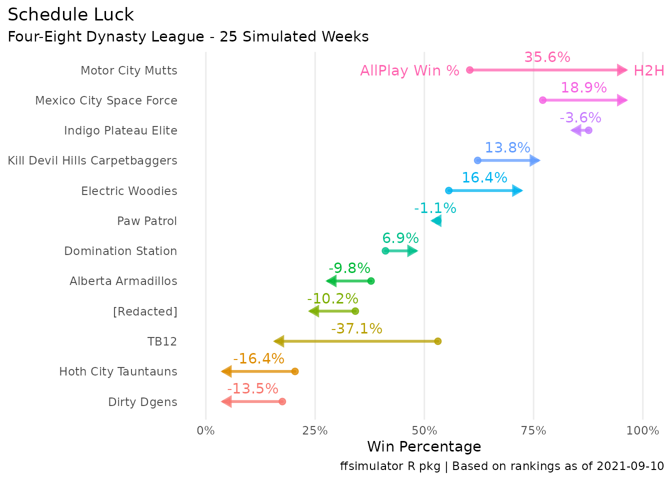
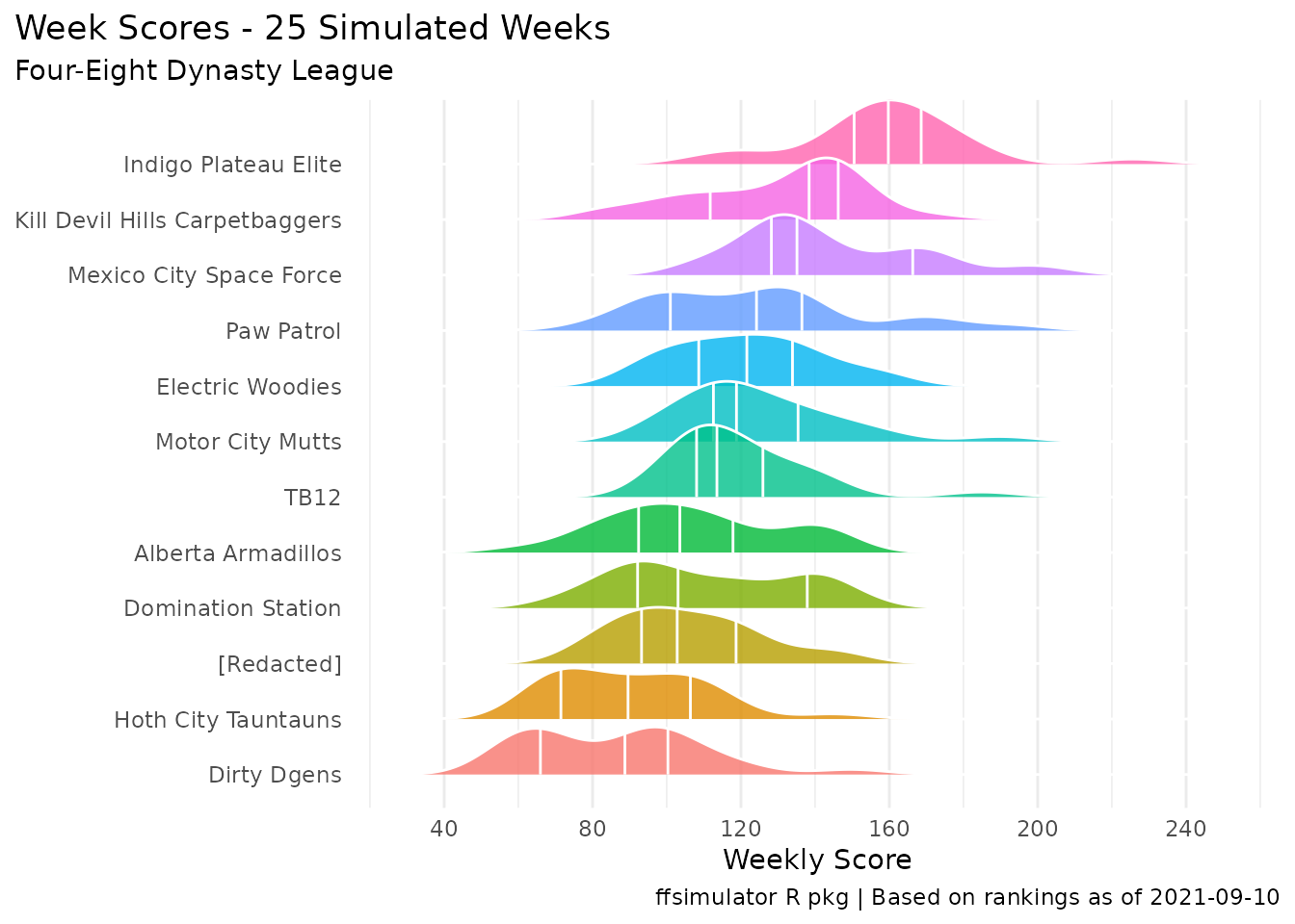
and the usual points distribution:
plot(foureight_sim_week, type = "points")
#> Picking joint bandwidth of 9.54